What does space already know
about a galaxy
before we look?

The Rotation Problem

Galaxies spin too fast. The outer stars move as though held by invisible hands — far beyond what visible matter should allow. According to Newtonian dynamics, velocity should fall off with distance. Instead, rotation curves flatten and hold. This discrepancy is one of modern astrophysics's most enduring puzzles.

In 1933, Fritz Zwicky identified excess motion in galaxy clusters and proposed unseen mass — dunkle Materie. In the 1970s, Vera Rubin confirmed the effect in individual spirals with unmistakable precision. The mainstream response has been to invoke a massive dark matter halo surrounding each galaxy. An alternative, MOND, modifies dynamics at low accelerations. Both approaches reproduce the general shape of rotation curves — but neither arises from first principles, and neither connects the phenomenon to a fundamental constant of nature.

"If I could have my pick, I would like to learn that Newton's laws must be modified in order to correctly describe gravitational interactions at large distances." — Vera Rubin, 1980

Spatial-Causal Geometry offers a third path — not added mass, not modified force, but a change in the question itself.

The Geometric Perspective

In SCG, space is not empty. It has structure: a scalar density field ρ(x) whose gradients generate all apparent forces. Acceleration is not caused by mass pulling — it emerges from curvature in the log of this field:

This is not a force law. It is a statement about geometry. Where the field curves, structures respond. Where it is flat, nothing moves. The geometry of space itself drives the motion of stars.

From this field equation, circular motion in a disk galaxy follows directly. A star at radius r within a causal domain where the density field has local exponent B_i will orbit with velocity:

When B_i ≈ 1, velocity is approximately flat — the canonical "flat rotation curve." When B_i < 1, velocity rises. When B_i > 1, it falls. The full variety of observed galactic rotation profiles emerges naturally from local variations in the causal-density exponent — no free parameters, no dark matter.

The Invariant: γ_cause = 1.216

The critical question in applying this framework to galaxies is: where do the domain boundaries sit? What determines where one kinematic regime ends and another begins?

The answer is a universal geometric constant. Derived originally from the causal closure condition of transverse electromagnetic oscillations — the requirement that a photon's internal structure remain coherent across its propagation — the causal ratio γ_cause defines the ratio between causal path length L and propagation wavelength λ in any c-bounded system:

Applied to a galaxy, this invariant defines the radial width of each causal domain — the distance over which one geometric closure of the causal field occurs. The spacing rule is:

The same constant that governs a photon's internal oscillation also governs the coherence scale of a rotating disk tens of kiloparsecs across. This scale invariance — from quantum to galactic — is a central claim of SCG.

How the Pipeline Works

The processing pipeline applies the γ_cause domain spacing law to each galaxy in the SPARC sample and reads the local velocity structure within each pre-defined domain. No global optimization is performed. The sequence for each galaxy is:

1. Compute domain boundaries from Δr_i = γ_cause · √r_i, starting at the galaxy's innermost observed radius. Boundaries are fixed before any velocity data is examined.
2. Extract local slope B_i within each domain via least-squares regression on log(r) vs. log(v). B_i is a diagnostic — it describes the curvature of the density field in that domain. It is read, not fitted.
3. Anchor the amplitude locally at the domain's median-radius data point: A_i = v* / r*^(1−B_i)/2. No global scaling constant is introduced.
4. Compute per-domain RMSD between the predicted and observed velocities. Domains with fewer than 3 data points are flagged as under-sampled and excluded from statistics.

Why a Single Curve Is the Wrong Question

The conventional approach to galactic rotation curve fitting draws one smooth function across the entire disk and minimizes the residuals globally. This seems natural — but it rests on an assumption the data do not support: that a galaxy is a single, geometrically uniform system from center to edge.

SCG says otherwise. Each causal domain is a geometrically distinct region of the galaxy — a zone in which the scalar density field has its own local curvature character, its own exponent B_i, its own kinematic identity. The domain boundaries at Δr_i = γ_cause · √r_i are not arbitrary breakpoints chosen to improve a fit. They are where the causal field undergoes a geometric closure — where one coherence scale ends and the next begins. Crossing a domain boundary means entering physically distinct territory.

Fitting a single curve across causally separate domains is therefore not merely imprecise — it is categorically the wrong thing to do. It is like measuring the slope of a road that bends several times and reporting a single average gradient. You will get a number, but it describes the average of turns you refused to acknowledge, not the road itself. The residuals of such a fit are not noise. They are the geometry you flattened out.

This is why the SCG pipeline treats each domain independently. B_i is read locally within each pre-defined region. The amplitude is anchored locally. The RMSD is computed per domain. The galaxy is not forced into a single geometric identity it does not possess. It is allowed to be — as it actually is — a succession of distinct causal regimes, each described by the same invariant law operating at a different local curvature.

Two Galaxies, One Lesson

The most important insight from applying the γ_cause pipeline at scale is this: high RMSD does not mean the model failed. It means the galaxy experienced something. The invariant faithfully describes systems in causal equilibrium. When a galaxy has been disturbed — by a merger, a tidal interaction, a disk warp — its velocity field carries the memory of that event, and the RMSD reads it.

Two galaxies illustrate this precisely. Both have 100% valid domains — the data is dense and well-sampled in both cases. The difference is not in the measurement. It is in the history of the galaxy itself.

DDO 161 In Equilibrium

0.62 km/s RMSD

6 / 6 Valid domains

1.00 Validity ratio

12.8 kpc Radial span

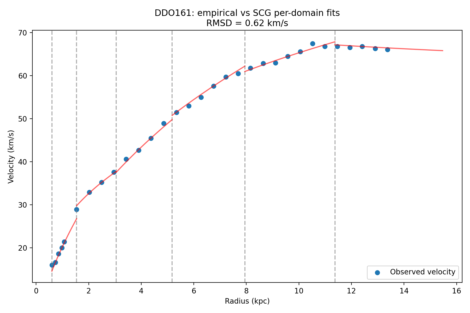
A late-type dwarf irregular, geometrically simple and kinematically quiet. All six γ_cause domains are fully sampled. The predicted boundaries align with the observed slope transitions, and the velocity curve follows the causal geometry without deviation. This is what equilibrium looks like.

NGC 4013 Historical Disturbance

3.74 km/s RMSD

6 / 6 Valid domains

1.00 Validity ratio

25.5 kpc Radial span

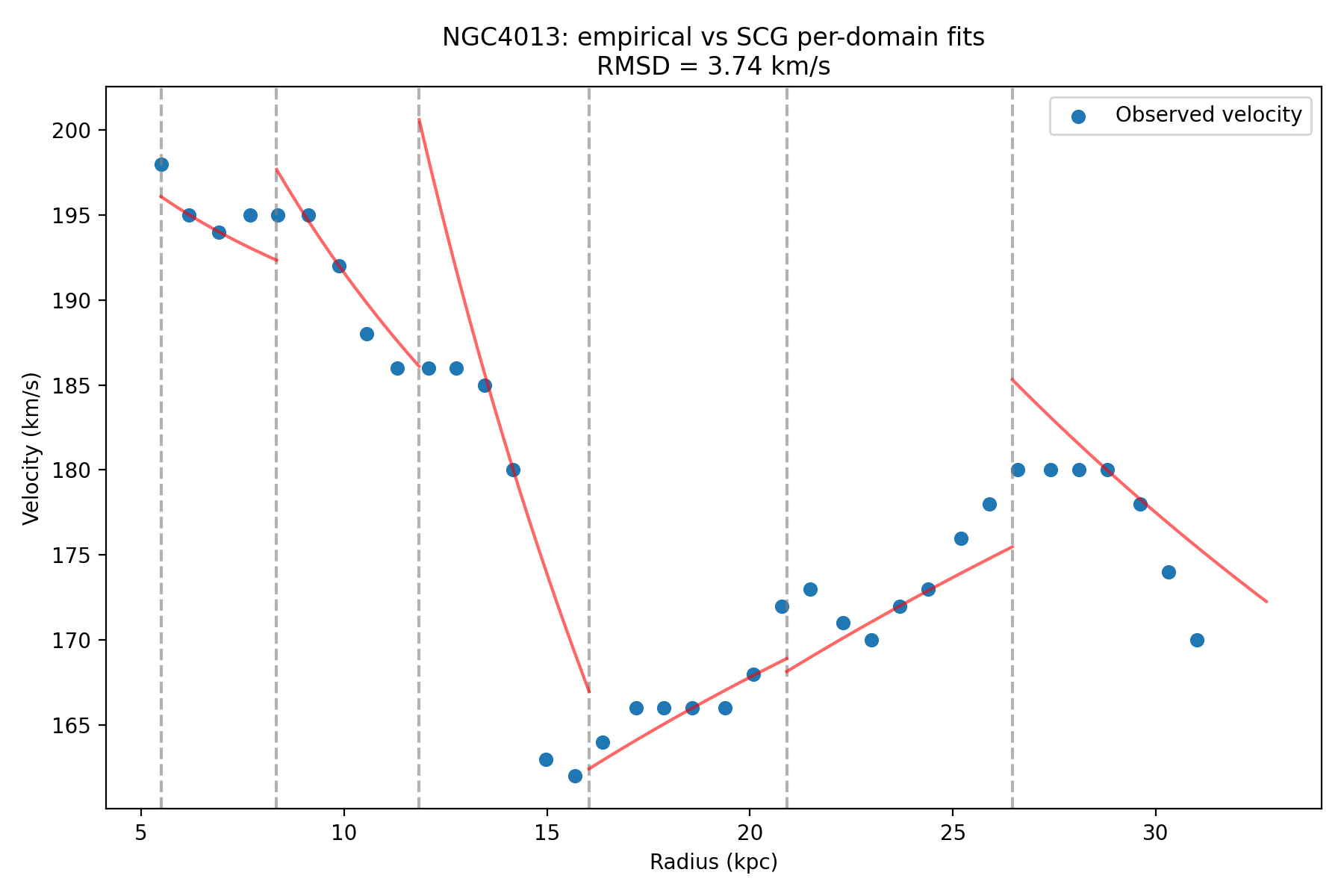
NGC 4013 is a well-documented warped-disk galaxy. Its outer disk has been displaced from the plane, almost certainly by a past tidal interaction. All six domains are fully sampled — the data quality is excellent. The elevated RMSD reflects a characteristic V-shaped velocity dip at 14–16 kpc that no smooth causal-density field can follow, because the disk itself is no longer in equilibrium. The γ_cause boundaries are correctly placed. The galaxy is not.

The contrast is the point. Both galaxies have identical data quality by the validity filter. The difference between RMSD = 0.62 and RMSD = 3.74 is not a modeling artifact — it is a record of galactic history. The SCG pipeline does not just fit rotation curves. It classifies them: systems in causal equilibrium versus systems that have been disturbed and are still carrying the signature of that disturbance in their kinematics.

This gives RMSD a second meaning in the SCG context. It is not only a goodness-of-fit statistic. It is a kinematic disturbance index. Galaxies with elevated RMSD and high validity ratios are candidates for morphological follow-up — warped disks, recent mergers, tidal interactions. The geometry points the way.

Global Results: 145 Galaxies

The central result is the alignment of pre-computed domain boundaries with observed kinematic transitions across all 145 galaxies. These boundaries are placed by the causal spacing law Δr_i = γ_cause√r_i before any velocity data is consulted. The fact that observed slope reversals fall systematically at these pre-computed radii — across galaxies spanning four orders of magnitude in baryonic mass — is the primary claim of this framework.

Within each domain, the locally reconstructed velocity profiles achieve a median root-mean-square deviation of 1.06 km/s and a mean of 1.73 km/s. These low residuals confirm that the predicted boundaries correctly identified the natural kinematic structure of each galaxy. They are not a claim of fitting power — they are the answer to: did the boundaries work?

Comparison with other approaches

Note: The table below compares RMSD values across frameworks for context only. Dark matter and MOND models make forward dynamical predictions with globally constrained parameters. SCG places domain boundaries before any velocity data is consulted and reads local geometry within those boundaries. These are different operations and RMSD values are not directly comparable across them. The unique claim of SCG — that kinematic transition locations are predicted by γ_cause alone — has no equivalent in any other framework listed here.

The correlation between RMSD and domain count is slightly positive (r = +0.25), confirming that the per-domain amplitude anchoring does not artificially reduce residuals. If local normalization were driving the fit quality, the correlation would be strongly negative. More complex galaxies produce slightly higher residuals — exactly what a genuine geometric model predicts.

All 145 Galaxies

Click any row's View link to display the SCG domain reconstruction for that galaxy. Sort by any column. Use the filter buttons to focus on specific populations.

Pipeline Code (Python)

The complete pipeline. Domain boundaries are computed from γ_cause before any velocity data is examined. The local slope B_i is read, not fitted. No global optimization is performed.

import pandas as pd
import numpy as np
import matplotlib.pyplot as plt
from pathlib import Path

# === CONFIG ===
gamma_cause = 1.216
skiprows = 3
colnames = ["r_kpc", "Vobs", "errV", "Vgas", "Vdisk", "Vbul", "SBdisk", "SBbul"]
out_dir = Path("gamma_cause_results")
out_dir.mkdir(exist_ok=True)

def load_rotation_file(filepath):
    df = pd.read_csv(filepath, delim_whitespace=True, comment="#",
                     skiprows=skiprows, names=colnames)
    return df[["r_kpc", "Vobs"]].dropna().sort_values("r_kpc")

def compute_domain_edges(r_min, r_max, gamma=gamma_cause):
    """
    Pre-compute domain boundaries from the causal spacing law:
        Δr_i = γ_cause · √r_i
    Boundaries are fixed before any velocity data is consulted.
    """
    edges = [r_min]
    r = r_min
    while r < r_max:
        dr = gamma * np.sqrt(max(r, 0.5))
        r += dr
        edges.append(r)
    return edges

def compute_Bs(df, edges):
    """
    Read the local causal-density exponent B_i within each pre-defined domain.
    B_i = 1 - 2·(d ln v / d ln r)  — diagnostic, not fitted.
    """
    rows = []
    for i in range(len(edges)-1):
        r_lo, r_hi = edges[i], edges[i+1]
        dom = df[(df["r_kpc"] >= r_lo) & (df["r_kpc"] <= r_hi)]
        if len(dom) < 2:
            B = np.nan
        else:
            m, _ = np.polyfit(np.log(dom["r_kpc"]), np.log(dom["Vobs"]), 1)
            B = 1 - 2 * m
        rows.append({"i": i, "r_lo": r_lo, "r_hi": r_hi, "B": B, "n": len(dom)})
    return pd.DataFrame(rows)

def rmsd(obs, model):
    return np.sqrt(np.nanmean((obs - model) ** 2))

# --- main loop ---
summary_rows = []

for file in Path("./SPARC_Data").glob("*.dat"):
    name = file.stem.split("_rotmod")[0]
    try:
        df = load_rotation_file(file)
        edges = compute_domain_edges(df["r_kpc"].min(), df["r_kpc"].max())
        Bdf = compute_Bs(df, edges)
        v_pred_all, v_obs_all = [], []
        valid_domains = 0

        fig, ax = plt.subplots(figsize=(9, 6))
        ax.scatter(df["r_kpc"], df["Vobs"], s=35, color="tab:blue",
                   label="Observed velocity")
        for r_edge in edges:
            if r_edge <= df["r_kpc"].max():
                ax.axvline(r_edge, color="gray", linestyle="--", alpha=0.6)

        for _, row in Bdf.iterrows():
            if np.isnan(row["B"]) or row["n"] < 3:
                continue
            valid_domains += 1
            r_lo, r_hi, B = row["r_lo"], row["r_hi"], row["B"]
            dom = df[(df["r_kpc"] >= r_lo) & (df["r_kpc"] <= r_hi)]
            # Amplitude anchored at median-radius data point — no global fitting
            anchor = dom.iloc[len(dom) // 2]
            r_star, v_star = anchor["r_kpc"], anchor["Vobs"]
            p = (1 - B) / 2
            if r_star <= 0:
                continue
            A_i = v_star / (r_star ** p)
            r_s = np.linspace(r_lo, r_hi, 200)
            v_s = A_i * (r_s ** p)
            ax.plot(r_s, v_s, color="red", alpha=0.6, lw=1.5)
            v_model_interp = np.interp(dom["r_kpc"], r_s, v_s)
            v_pred_all.extend(v_model_interp)
            v_obs_all.extend(dom["Vobs"])

        galaxy_rmsd = (rmsd(np.array(v_obs_all), np.array(v_pred_all))
                       if len(v_obs_all) > 0 else np.nan)

        ax.set_xlabel("Radius (kpc)")
        ax.set_ylabel("Velocity (km/s)")
        ax.set_title(f"{name}: empirical vs SCG per-domain fits\n"
                     f"RMSD = {galaxy_rmsd:.2f} km/s  |  "
                     f"{valid_domains}/{len(Bdf)} valid domains")
        ax.legend()
        fig.tight_layout()
        fig.savefig(out_dir / f"{name}_with_SCG_domains.png", dpi=200)
        plt.close(fig)

        summary_rows.append({
            "galaxy": name,
            "n_domains_total": len(Bdf),
            "n_domains_valid": valid_domains,
            "r_min": df["r_kpc"].min(),
            "r_max": df["r_kpc"].max(),
            "r_span": df["r_kpc"].max() - df["r_kpc"].min(),
            "RMSD_kms": galaxy_rmsd
        })

        print(f"✅ {name}: RMSD={galaxy_rmsd:.2f} km/s  "
              f"({valid_domains}/{len(Bdf)} valid domains)")

    except Exception as e:
        print(f"⚠️  {name}: failed ({e})")

summary_df = pd.DataFrame(summary_rows)
summary_df.to_csv("SCG_summary.csv", index=False)
print(f"\n📊 Summary saved to SCG_summary.csv")

References